Models of Learning

• Introduction

  1. Task description

• Reinforcement Learning

  1. Theory
     • Rescorla-Wagner
     • SoftMax
  2. Data plotting
  3. Simulation
     • Example participants
     • More participants
     • Explore Parameters
     • Grid Search
     • Marginal distributions
     • Summary values
  4. Real data
     • Fit the data
     • Statistical inference
  5. Review
     • Modelling how-to

• Bayesian Learning

  1. Coin tossing
     • Probability
     • Likelihood
     • Uncertainty
     • Learning
     • Review
  2. Bandit task
     • Updating
     • Transition function
     • Learning rate

Developed by
Jill O'Reilly
Hanneke den Ouden
-August 2015

Transition Function

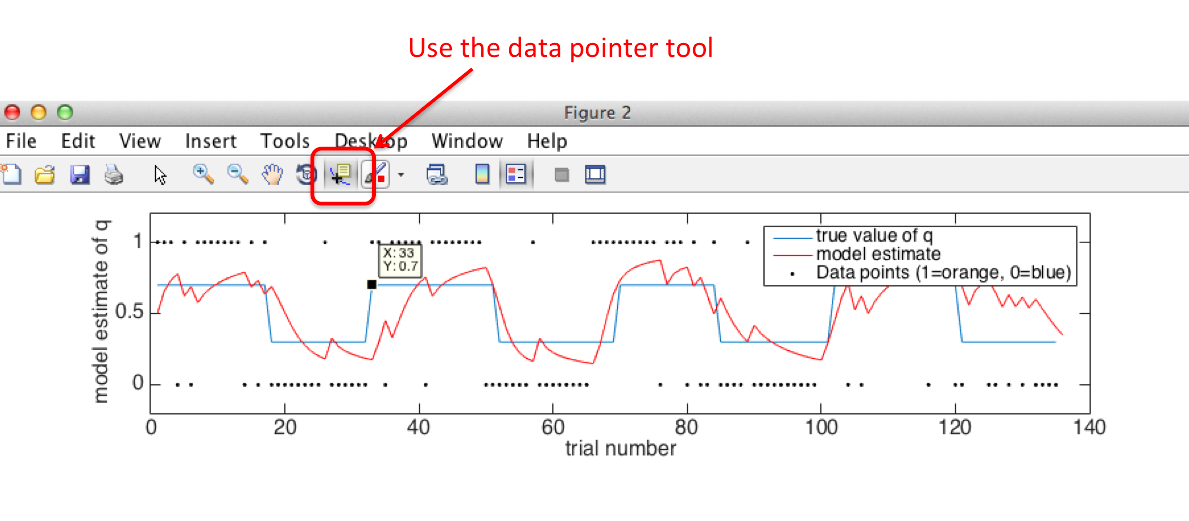
As you can see from figure 2, the model tracks the true value of q quite well as it changes over time.

To make this work, we had to modify slightly the plan presented in part 1.

As you may recall, when we did the sequential learning with Bayes' Theorem at the end of Part 1, we pooled our knowledge across trials by using the posterior from trial t became the prior for trial t+1

Built into that process is the assumption that the q we are estimating on trial t+1 is the same as the q we were estimating on trial t, ie q_t=q_t+1

That is fine if we are trying to estimate a parameter that doesn't change, like the probability that a given coin comes up heads, but is clearly not a correct assumption in the reversal learning task.

To account for the possibility that q_t ≠ q_t+1, ie there has been a reversal, we build in a leaky transition function. What does this mean?

• Instead of using the posterior from trial t as the prior for trial t+1 directly, we modify it slightly by adding a uniform probability distribution over all possible values of q

  ?

  

• So q_t+1 can have either
  • The same distribution as q_t+1
  • A uniform distribution
• The model has to infer which one is correct.

Take a look at Figure 4. This shows how the probability distribution over q changes following a reversal.

?

• Have a look at the trial numbers on each subplot and identify which trials this corresponds to on Figure 2.
• Initially, the model thinks q is around 0.8 - that is p(orange rewarded) is about 0.8
• On which trial does the true reversal occur?

  ?

  33 - you can work this out from looking at the blue line in Figure 2. If you use the data point selector tool in Matlab, you can click on the line and it tells you exactly which point you are looking at.

  

• Now look at how the probability distribution changes in the trials following the reversal, in Figure 4. You can see the model gradually changing its mind!

To understand what would happen if we didn't use this leaky transition function, go to line 16 of the Matlab script and set the value of H to 0, then run the script again.

Because the model assumes q is fixed over all trials, after it has seen several reversals, it ends up thinking the probability each option is rewarded is 50%! Clearly this is not a good model of the environment.

We can think about the leaky transition function as including a little bit of uncertainty about q on each trial. Without the leak, uncertainty goes down and down as more data points are seen, and the model can't learn any more.

• H is the hazard rate used by the model - the model 'believes' that there is a constant reversal probability, and on any given trial, the probability of reversal is H
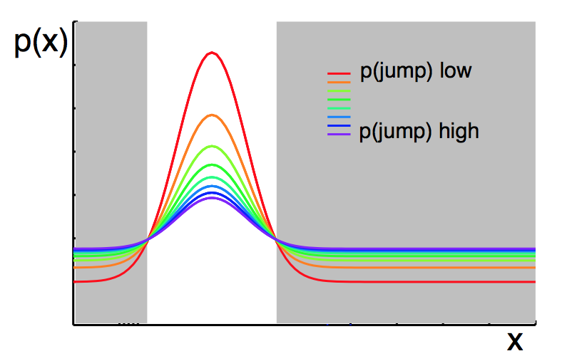
• In practice, H determines how much the prior on trial t+1 depends on the posterior from trial t, and how much it reflects the uniform distribution.

  ?

  The coloured lines represent the prior on trial t+1, given a certain posterior on trial t and a varying Hazard rate in the model.

  

Try setting H to different values and running the model again.

• What happens when H is very high, eg 4/5?

  ?

  The model learns very quickly about reversals, but it is also unstable during the blocks - so if the model thinks orange is the rewarded side, one trial on which blue is rewarded instead changes its beliefs a lot.

• What happens when H is very low, eg 1/50?

  ?

  The model is stable during each block, but learns very slowly following reversals.

►►►