Models of Learning

• Introduction

  1. Task description

• Reinforcement Learning

  1. Theory
     • Rescorla-Wagner
     • SoftMax
  2. Data plotting
  3. Simulation
     • Example participants
     • More participants
     • Explore Parameters
     • Grid Search
     • Marginal distributions
     • Summary values
  4. Real data
     • Fit the data
     • Statistical inference
  5. Review
     • Modelling how-to

• Bayesian Learning

  1. Coin tossing
     • Probability
     • Likelihood
     • Uncertainty
     • Learning
     • Review
  2. Bandit task
     • Updating
     • Transition function
     • Learning rate

Developed by
Jill O'Reilly
Hanneke den Ouden
-August 2015

Summary values for α and β

The distributions over α and β give us a full picture of these parameters: a probability for each value in the bin, that that parameter value generated the observed data.

However, for our analysis we usually we want a single estimate for α and β.

How would you go about obtaining this from the distributions plotted on the previous page?

?

The simplest option is to take the maximum (or peak) of the distribution. This is what we call the maximum likelihood estimate. However, this ML estimate disregards the fact that we have more information about the estimated parameter.

A usually more reliable and stable estimate is the mean of the distribution, or the value of each bin multiplied with the probability of that value. This is called the expected value (EV).

Let's have a look at how well this model is performing. In the original trial-by-trial dataplot, we now added the estimated choice probabilities (in turquoise)

?

simulate-refit results: trial-by-trial choice probabilities

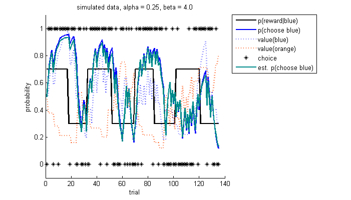
Overall, the estimated choice probabilities in turquoise are matching the original, simulated choice probabilities (in blue) very well. You could also add the estimated values of each of the stimuli here and compare how they match the simulated values.

From this plot, it is hard to quantify how well the estimated probabilities are matching the simulated choice probabilities. We will next look at the correlation of the original, simulated choice probabilities, and correlate these with the choice probabilities that we obtained from both the maximuml likelihood and expected value estimates:

?

simulate-refit results: choice probability correlogram

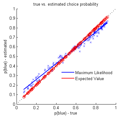
Correlation of simulated probability of choosing blue with 1) maximum likelihood estimate (ML; blue) and 2) expected value estimate (EV; red) of the choice probabilities For perfect performance, the estimated and true probabilities are identical, ie on the unity line (black dashed). Both ML and EV estimates are doing very well, though in this single simulation/refit it looks like the EV estimate is performing slightly better than the ML.

To quantify whether the ML or EV is doing better, you would have to run many simulations for a range of parameter values, and compare how much the ML and EV predicted choice probabilities deviate from the simulated choice probabilities.

Below, we will do something slightly different, and have a look at how good both the ML and the EV estimates, are at recovering parameter values for α and β across a large number of iterations.

Because estimating the parameters takes a bit longer than just generating data, we'll go for a slightly lower subject number, let's do 20 for each of the 2 conditions.

Set the following....

subjects = 1:40;
simulate = true;
fitData = true;
plotIndividual = false;

...save, and run!

You now see both the probability density functions (PDFs) for each of the parameter across all subjects, separately for each condition.

?

Probability distributions for each subject and each parameter.

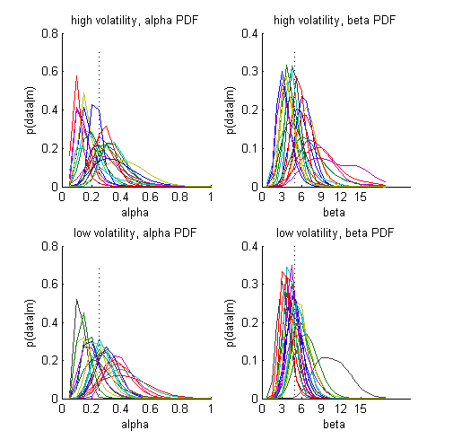
Each coloured line is an individual subject
Dashed vertical line indicates the parameter value used to simulate the data

• If the distributions are 'peaked', then we have high confidence in the estimate of the parameters
• If the distributions are very broad, our estimates are less precise
• Note that for some subjects, the tails of the distributions are cut off, or 'hit the bounds' of our grid. This might mean that you have to enlarge the grid to cover the full parameter space.
• Remember the true values of α and β (the ones we put into the simulation) are 0.25 and 4.
  • How well is the model doing at recovering these parameter values?

We can also view these aggregated across all subjects

?

Summary of parameter values for 20 subjects

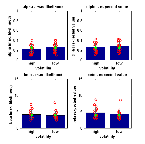
LEFT: maximum likelihood estimate (distribution peak), RIGHT: expected value (distribution mean). Mean across simulations (blue) ± standard deviation (grey); individual estimates from each simulation (red); 'ground truth' (green) - i.e. the parameter values used to simulate the data.

What conclusions can we draw from these plots?

?

1. On average, the parameters are estimated well by the model: The green dot is close to the height of the blue bars. However, there is a lot of variance in the estimates, despite all data being generated using the same parameter values.
   • Suggested exercise: Test how good the model is at recovering the parameters. For this, write a loop around the code to simulate multiple values of alpha and plot these against the true value. If the model is good at recovering the true parameters, the points on this scatterplot should be on the unity line.
2. The EV and ML estimates don't seem to differ much in terms of their performance.
   • Suggested exercise: Play around with reducing the bin size. Does the performance of the ML estimates change a lot? What about the EV estimates? Can you think of why?

►►►